Multilayer Perceptrons in Machine Learning
Neural networks are at the center of present day machine learning and artificial intelligence. Among the many sorts, multilayer perceptrons (MLPs) serve as a foundational building square for deep learning frameworks. This instructional exercise presents the concept of counterfeit neural networks, investigates how MLPs work, and strolls through key components like backpropagation and stochastic slope descent.
An artificial neural network (ANN) is a machine learning demonstrate motivated by the structure and work of the human brain’s interconnected organize of neurons. It comprises of interconnected hubs called artificial neurons, organized into layers. Data streams through the arrange, with each neuron preparing input signals and creating an yield flag that impacts other neurons in the network.
A multi-layer perceptron (MLP) is a sort of artificial neural network comprising of different layers of neurons. The neurons in the MLP ordinarily utilize nonlinear enactment capacities, permitting the network to learn complex designs in information. MLPs are critical in machine learning since they can learn nonlinear connections in information, making them effective models for tasks such as classification, regression, and design acknowledgment. In this instructional exercise, we might jump deeper into the nuts and bolts of MLP and get it its internal workings.
Basics of Neural Networks
Neural systems or manufactured neural systems are fundamental instruments in machine learning, powering many state-of-the-art calculations and applications over different spaces, counting computer vision, characteristic dialect preparing, robotics, and more.
A neural network consists of interconnected nodes, called neurons, organized into layers. Each neuron gets input signals, performs a computation on them utilizing an actuation work, and produces an yield flag that may be passed to other neurons in the arrange. An actuation work decides the yield of a neuron given its input. These capacities present nonlinearity into the organize, empowering it to learn complex designs in data.
The network is regularly organized into layers, beginning with the input layer, where information is presented. Taken after by covered up layers where computations are performed and at long last, the yield layer where forecasts or choices are made.
Neurons in adjoining layers are associated by weighted associations, which transmit signals from one layer to the another. The quality of these associations, spoken to by weights, decides how much impact one neuron’s yield has on another neuron’s input. Amid the preparing handle, the organize learns to alter its weights based on cases given in a preparing dataset. Moreover, each neuron regularly has an related predisposition, which permits the neuron to alter its yield threshold.
Neural systems are prepared utilizing strategies called feedforward propagation and backpropagation. During feedforward engendering, input information is passed through the organize layer by layer, with each layer performing a computation based on the inputs it gets and passing the result to the another layer.
Backpropagation is an calculation utilized to prepare neural systems by iteratively altering the network’s weights and inclinations in arrange to minimize the loss work. A misfortune work (too known as a fetched work or objective work) is a degree of how well the model’s expectations coordinate the genuine target values in the preparing information. The loss work quantifies the distinction between the anticipated yield of the show and the real yield, giving a flag that guides the optimization handle amid training.
The objective of preparing a neural arrange is to minimize this misfortune work by altering the weights and predispositions. The alterations are guided by an optimization calculation, such as angle plunge. We will return to a few of these points in more detail afterward on in this tutorial.
Types of Neural Networks
The ANN depicted on the right of the picture is a straightforward neural network called ‘perceptron’. It comprises of a single layer, which is the input layer, with different neurons with their possess weights; there are no covered up layers. The perceptron calculation learns the weights for the input signals in arrange to draw a direct choice boundary.

However, to illuminate more complicated, non-linear issues related to picture handling, computer vision, and common language preparing tasks, we work with deep neural networks.
Check out Datacamp’s Introduction to Deep Neural Systems instructional exercise to learn more approximately profound neural systems and how to build one from scratch utilizing TensorFlow and Keras in Python. If you would incline toward to utilize R dialect instep, Datacamp’s Building Neural Network (NN) Models in R has you covered.
There are a few sorts of ANN, each outlined for particular errands and structural requirements. Let’s briefly examine a few of the most common sorts before jumping deeper into MLPs next.
What Is a Multilayer Perceptron (MLP)?
Feedforward Neural Networks (FNN)
These are the simplest shape of ANNs, where data streams in one course, from input to yield. There are no cycles or circles in the arrange design. Multilayer perceptrons (MLP) are a sort of feedforward neural network.
Recurrent Neural Systems (RNN)
In RNNs, associations between hubs frame coordinated cycles, permitting data to hold on over time. This makes them appropriate for assignments including consecutive information, such as time arrangement forecast, normal dialect preparing, and discourse recognition.
Convolutional Neural Systems (CNN)
CNNs are planned to viably handle grid-like information, such as pictures. They comprise of layers of convolutional channels that learn various leveled representations of highlights inside the input information. CNNs are broadly utilized in errands like picture classification, question discovery, and picture segmentation.
Long Short-Term Memory Networks (LSTM) and Gated Repetitive Units (GRU)
These are specialized sorts of repetitive neural systems planned to address the vanishing slope issue in conventional RNN. LSTMs and GRUs consolidate gated components to way better capture long-range conditions in successive information, making them especially compelling for errands like discourse acknowledgment, machine interpretation, and estimation analysis.
It is outlined for unsupervised learning and comprises of an encoder arrange that compresses the input information into a lower-dimensional inactive space, and a decoder arrange that remakes the unique input from the idle representation. Autoencoders are regularly utilized for dimensionality diminishment, information denoising, and generative modeling.
Generative Adversarial Networks (GAN)
GANs comprise of two neural systems, a generator and a discriminator, prepared at the same time in a competitive setting. The generator learns to produce engineered information tests that are unclear from genuine information, whereas the discriminator learns to recognize between genuine and fake tests. GANs have been broadly utilized for producing practical pictures, recordings, and other sorts of data.
A multilayer perceptron is a sort of feedforward neural arrange comprising of completely associated neurons with a nonlinear kind of actuation work. It is broadly utilized to recognize information that is not straightly separable.
MLPs have been broadly utilized in different areas, counting picture acknowledgment, normal language preparing, and discourse acknowledgment, among others. Their adaptability in engineering and capacity to surmised any work beneath certain conditions make them a principal building piece in deep learning and neural arrange inquire about. Let’s take a more profound jump into a few of its key concepts.
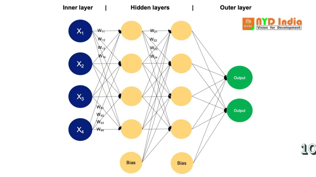
The input layer comprises of hubs or neurons that get the starting input information. Each neuron speaks to a include or measurement of the input information. The number of neurons in the input layer is decided by the dimensionality of the input data.
Between the input and yield layers, there can be one or more layers of neurons. Each neuron in a covered up layer gets inputs from all neurons in the past layer (either the input layer or another covered up layer) and produces an yield that is passed to the following layer. The number of covered up layers and the number of neurons in each covered up layer are hyperparameters that require to be decided amid the show plan phase.
This layer comprises of neurons that deliver the last yield of the organize. The number of neurons in the yield layer depends on the nature of the assignment. In twofold classification, there may be either one or two neurons depending on the activation work and speaking to the likelihood of having a place to one course; whereas in multi-class classification tasks, there can be numerous neurons in the yield layer.
Neurons in adjoining layers are completely associated to each other. Each association has an related weight, which decides the quality of the association. These weights are learned amid the preparing process.
In expansion to the input and covered up neurons, each layer (but the input layer) more often than not incorporates a predisposition neuron that gives a steady input to the neurons in the following layer. Bias neurons have their claim weight related with each association, which is moreover learned amid training.
The bias neuron viably shifts the enactment work of the neurons in the ensuing layer, permitting the arrange to learn an balanced or predisposition in the choice boundary. By altering the weights associated to the predisposition neuron, the MLP can learn to control the edge for actuation and superior fit the preparing data.
Note: It is critical to note that in the setting of MLPs, inclination can allude to two related but particular concepts: predisposition as a common term in machine learning and the inclination neuron (characterized over). In common machine learning, inclination alludes to the blunder presented by approximating a real-world issue with a disentangled demonstrate. Inclination measures how well the show can capture the fundamental designs in the information. A tall bias shows that the demonstrate is as well oversimplified and may underfit the information, whereas a low predisposition recommends that the demonstrate is capturing the basic designs well.
Typically, each neuron in the covered up layers and the yield layer applies an enactment work to its weighted whole of inputs. Common actuation capacities incorporate sigmoid, tanh, ReLU (Corrected Direct Unit), and softmax. These capacities present nonlinearity into the arrange, permitting it to learn complex designs in the data.
Feedforward and Backpropagation
MLPs are prepared utilizing the backpropagation calculation, which computes angles of a misfortune work with regard to the model’s parameters and overhauls the parameters iteratively to minimize the misfortune.
How a Multilayer Perceptron Works: Layer by Layer
In a multilayer perceptron, neurons process information in a step-by-step way, performing computations that include weighted sums and nonlinear changes. Let’s walk layer by layer to see the magic that goes within.
The input layer of an MLP gets input information, which may be highlights extracted from the input tests in a dataset. Each neuron in the input layer speaks to one feature.
Neurons in the input layer do not perform any computations; they essentially pass the input values to the neurons in the to begin with covered up layer.
The covered up layers of an MLP comprise of interconnected neurons that perform computations on the input data.
Each neuron in a covered up layer gets input from all neurons in the past layer. The inputs are duplicated by comparing weights, indicated as w. The weights decide how much impact the input from one neuron has on the yield of another.
In expansion to weights, each neuron in the covered up layer has an related bias, signified as b. The bias gives an extra input to the neuron, permitting it to alter its yield edge. Like weights, inclinations are learned amid training.
For each neuron in a covered up layer or the yield layer, the weighted whole of its inputs is computed. This includes duplicating each input by its comparing weight, summing up these items, and including the bias:
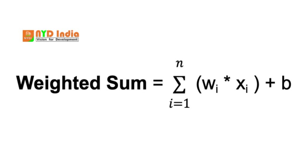
Where n is the add up to number of input associations, wi is the weight for the i-th input, and xi is the i-th input value.
The weighted entirety is at that point passed through an activation work, signified as f. The actuation work presents nonlinearity into the arrange, permitting it to learn and speak to complex connections in the information. The activation work decides the yield run of the neuron and its behavior in reaction to different input values. The choice of activation work depends on the nature of the assignment and the craved properties of the network.
The yield layer of an MLP produces the last forecasts or yields of the arrange. The number of neurons in the yield layer depends on the assignment being performed (e.g., twofold classification, multi-class classification, regression).
Each neuron in the yield layer gets input from the neurons in the final covered up layer and applies an enactment work. This activation work is usually diverse from those utilized in the covered up layers and produces the last yield esteem or prediction.
During the preparing prepare, the organize learns to alter the weights related with each neuron’s inputs to minimize the error between the predicted yields and the genuine target values in the preparing information. By altering the weights and learning the suitable actuation capacities, the arrange learns to approximate complex designs and connections in the information, empowering it to make exact expectations on unused, unseen samples.
This alteration is guided by an optimization calculation, such as stochastic angle plunge (SGD), which computes the slopes of a misfortune work with regard to the weights and overhauls the weights iteratively.
Stochastic Gradient Descent (SGD)
Initialization: SGD begins with an introductory set of show parameters (weights and predispositions) arbitrarily or utilizing a few predefined method.
Iterative optimization: The point of this step is to discover the least of a misfortune work, by iteratively moving in the heading of the steepest diminish in the function’s esteem. For each cycle (or age) of training:
Shuffle the preparing information to guarantee that the demonstrate doesn’t learn from the same designs in the same arrange each time.
Split the preparing information into mini-batches (little subsets of data).
For each mini-batch:
Compute the slope of the misfortune work with regard to the demonstrate parameters utilizing as it were the information focuses in the mini-batch. This angle estimation is a stochastic guess of the genuine gradient.
Update the show parameters by taking a step in the inverse course of the angle, scaled by the learning rate:
θₜ₊₁ = θₜ − η ∇J(θₜ)
Powered By
Where:
θₜ speaks to the show parameters (e.g., weights and biases) at cycle t
∇J(θₜ) is the angle of the misfortune work J with regard to the parameters at cycle t
η (estimated time of arrival) is the learning rate, which controls the step measure amid optimization
Direction of plunge: The angle of the misfortune work shows the heading of the steepest rising. To minimize the misfortune work, angle plunge moves in the inverse course, towards the steepest descent.
Learning rate: The step estimate taken in each emphasis of angle plunge is decided by a parameter called the learning rate, indicated over as n. This parameter controls the measure of the steps taken towards the least. If the learning rate is as well little, meeting may be moderate; if it is as well expansive, the calculation may waver or diverge.
Convergence: Rehash the prepare for a settled number of cycles or until a merging model is met (e.g., the alter in misfortune work is underneath a certain threshold).
Stochastic angle plunge upgrades the show parameters more habitually utilizing littler subsets of information, making it computationally effective, particularly for huge datasets. The haphazardness presented by SGD can have a regularization impact, avoiding the demonstrate from overfitting to the preparing information. It is moreover well-suited for online learning scenarios where modern information gets to be accessible incrementally, as it can upgrade the show rapidly with each modern information point or mini-batch.
However, SGD can too have a few challenges, such as expanded commotion due to the stochastic nature of the slope estimation and the require to tune hyperparameters like the learning rate. Different expansions and adjustments of SGD, such as mini-batch stochastic angle plunge, energy, and versatile learning rate strategies like AdaGrad, RMSProp, and Adam, have been created to address these challenges and progress merging and performance.
You have seen the working of the multilayer perceptron layers and learned almost stochastic angle plunge; to put it all together, there is one final subject to plunge into: backpropagation.
Backpropagation
Backpropagation is brief for “backward engendering of errors.” In the setting of backpropagation, SGD includes upgrading the network’s parameters iteratively based on the angles computed amid each group of preparing information. Instep of computing the slopes utilizing the whole preparing dataset (which can be computationally costly for huge datasets), SGD computes the slopes utilizing little irregular subsets of the information called mini-batches. Here’s an diagram of how backpropagation calculation works:
Forward pass: Amid the forward pass, input information is encouraged into the neural organize, and the network’s yield is computed layer by layer. Each neuron computes a weighted whole of its inputs, applies an actuation work to the result, and passes the yield to the neurons in the another layer.
Loss computation: After the forward pass, the network’s yield is compared to the genuine target values, and a misfortune work is computed to degree the inconsistency between the anticipated yield and the real output.
Backward pass (angle calculation): In the in reverse pass, the slopes of the misfortune work with regard to the network’s parameters (weights and predispositions) are computed utilizing the chain run the show of calculus. The slopes speak to the rate of alter of the misfortune work with regard to each parameter and give data around how to alter the parameters to diminish the loss.
Parameter overhaul: Once the slopes have been computed, the network’s parameters are overhauled in the inverse course of the angles in arrange to minimize the misfortune work. This upgrade is regularly performed utilizing an optimization calculation such as stochastic angle plunge (SGD), that we talked about earlier.
Iterative prepare: Steps 1-4 are rehashed iteratively for a settled number of ages or until meeting criteria are met. Amid each cycle, the network’s parameters are balanced based on the angles computed in the in reverse pass, continuously decreasing the misfortune and moving forward the model’s performance.
Data Preparation for MLPs
Preparing information for preparing an MLP includes cleaning, preprocessing, scaling, part, organizing, and possibly indeed expanding the information. Based on the actuation capacities utilized and the scale of the input highlights, the information might require to be standardized or normalized. Testing with diverse preprocessing methods and assessing their affect on demonstrate execution is frequently vital to decide the most reasonable approach for a specific dataset and task.
Data cleaning and preprocessing
Handle lost values: Evacuate or ascribe lost values in the dataset.
Encode categorical factors: Change over categorical factors into numerical representations, such as one-hot encoding.
Standardization or normalization: Rescale the highlights to a comparable scale to guarantee that the optimization handle meets efficiently.
Standardization (Z-score normalization): Subtract the cruel and partition by the standard deviation of each include. It centers the information around zero and scales it to have unit variance.
Normalization (Min-Max scaling): Scale the highlights to a settled extend, ordinarily between 0 and 1, by subtracting the least esteem and partitioning by the extend (max-min).
To learn more around include scaling, check out Datacamp’s Include Building for Machine Learning in Python course.
Train-validation-test split
Split the dataset into preparing, approval, and test sets. The preparing set is utilized to prepare the demonstrate, the approval set is utilized to tune hyperparameters and screen show execution, and the test set is utilized to assess the last model’s execution on concealed data.
Ensure that the information is in the suitable organize for preparing. This may include reshaping the information or changing over it to the required information sort (e.g., changing over categorical factors to numeric).
Optional information augmentation
For assignments such as picture classification, information increase methods such as revolution, flipping, and scaling may be connected to increment the differences of the preparing information and move forward demonstrate generalization.
Normalization and enactment functions
The choice between standardization and normalization may depend on the actuation capacities utilized in the MLP. Enactment capacities like sigmoid and tanh are delicate to the scale of the input information and may advantage from standardization. On the other hand, actuation capacities like ReLU are less delicate to the scale and may not require standardization.
Implementation Tips and Best Practices
Implementing a MLP includes a few steps, from information preprocessing to show preparing and assessment. Selecting the number of layers and neurons for a MLP includes adjusting demonstrate complexity, preparing time, and generalization execution. There is no one-size-fits-all reply, as the ideal design depends on components such as the complexity of the errand, the sum of accessible information, and computational assets. In any case, here are a few common rules to consider when actualizing MLP:
Begin with a straightforward design and slowly increment complexity as required. Begin with a single covered up layer and a little number of neurons, and at that point test with including more layers and neurons if necessary.
2.Errand complexity
For basic errands with generally moo complexity, such as parallel classification or relapse on little datasets, a shallow engineering with less layers and neurons may suffice.
For more complex errands, such as multi-class classification or relapse on high-dimensional information, more profound designs with more layers and neurons may be essential to capture perplexing designs in the data.
3.Information preprocessing
Clean and preprocess your information, counting taking care of lost values, encoding categorical factors, and scaling numerical features.
Split your information into preparing, approval, and test sets to assess the model’s performance.
4.Initialization
Initialize the weights and predispositions of your MLP suitably. Common initialization procedures incorporate irregular initialization with little weights or utilizing methods like Xavier or He initialization.
5.Experimentation
Ultimately, the best approach is to try with diverse structures, changing the number of layers and neurons, and assess their execution empirically.
Use procedures such as cross-validation and hyperparameter tuning to efficiently investigate distinctive designs and discover the one that performs best on the assignment at hand.
6.Training
Train your MLP utilizing the preparing information and screen its execution on the approval set.
Experiment with diverse bunch sizes, number of ages, and other hyperparameters to discover the ideal preparing settings.
7.Optimization algorithm
Visualize preparing advance utilizing measurements such as misfortune and precision to analyze issues and track merging.
Experiment with distinctive learning rates and consider utilizing procedures like learning rate plans or versatile learning rates.
Be cautious not to overfit the show to the preparing information by presenting superfluous complexity.
Use strategies such as regularization (e.g., L1, L2 regularization), dropout, and early halting to anticipate overfitting and make strides generalization performance.
Tune the regularization quality based on the model’s execution on the approval set.
Monitor the model’s execution on a isolated approval set amid preparing to survey how changes in engineering influence performance.
Evaluate the prepared demonstrate on the test set to evaluate its generalization performance.
Use measurements such as exactness, misfortune, and approval blunder to assess the model’s execution and direct building decisions.
Experiment with diverse structures, hyperparameters, and optimization techniques to progress the model’s performance.
Iterate on your usage based on experiences picked up from preparing and assessment results.
Final Thought
Multilayer perceptrons speak to a principal and flexible lesson of fake neural systems that have essentially contributed to the progression of machine learning and fake insights. Through their interconnected layers of neurons and nonlinear enactment capacities, MLPs are competent of learning complex designs and connections in information, making them well-suited for a wide extend of errands. The history of MLPs reflects a travel of investigation, disclosure, and development, from the early perceptron models to the present day profound learning models that control numerous state-of-the-art frameworks today.
In this article, you’ve learned the essentials of manufactured neural systems, centered on multilayer perceptrons, learned approximately stochastic angle plummet and backpropagation. If you are interested in getting hands-on involvement and utilizing profound learning strategies to illuminate real-world challenges, such as anticipating lodging costs, building neural systems to show pictures and content – we exceedingly prescribe taking after Datacamp’s Keras tool compartment track.
Working with Keras, you’ll learn approximately neural systems, profound learning demonstrate workflows, and how to optimize your models. Datacamp moreover has a Keras deceive sheet that can come in helpful!